Fragmentation#

Fragmentation analysis uses a Fixed Observation Scale (FOS) approach to compute foreground pattern indices within a user-defined moving window, which is a square neighbourhood of W × W pixels that is centred on each foreground pixel in the raster, one at a time. The window size W defines the side length of this square and must be an odd integer (e.g., 3, 5, 27) so that the centre pixel is unambiguously defined. As the window moves across the map, the fragmentation index is computed from all pixels within the window and assigned to the centre pixel. Larger windows capture broader landscape context but smooth local detail; smaller windows preserve fine-grained spatial patterns but are more sensitive to local noise. The choice of W determines the Fixed Observation Scale (FOS) at which fragmentation is measured.

To compute the foreground fragmentation, three methods are available:

FAD (Foreground Area Density): proportion of foreground pixels relative to the total number of window pixels.
FAC (Foreground Area Clustering): proportion of foreground–foreground adjacencies relative to all adjacencies. Supports 4- and 8-connectivity.
FED (Foreground Edge Density): weighted edge density where FG-FG pairs score 1.0, FG-BG pairs score 0.5, and BG-BG pairs score 0.0. Supports 4- and 8-connectivity.

Further details about Fragmentation analysis are available in the Connectivity/Fragmentation product sheet.

FAD: Foreground Area Density#

FAD computes the proportion of foreground pixels within the moving window relative to the total number of pixels in the window. It provides a direct measure of how much foreground (e.g., forest) is present in the local neighbourhood of each pixel. The denominator is always the total window area (W²), making FAD a pure area-based metric independent of pixel arrangement.

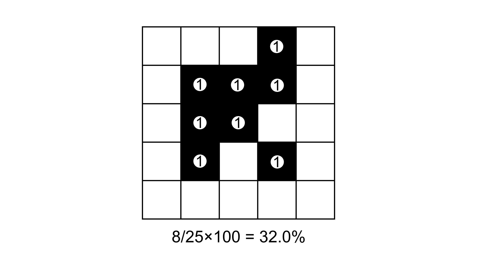
\[FAD = \frac{\text{number of foreground pixels}}{\text{total pixels}} \times 100\]

FAD method — FAD computation example on a 5×5 binary input map (black = foreground). The window contains 25 pixels of which 13 are foreground. Each foreground pixel contributes 1 to the numerator (shown as value “1” in the circles).#

FAC: Foreground Area Clustering#

FAC computes the proportion of foreground–foreground edges within the moving window relative to the total number of pixel pair edges. Unlike FAD, which only measures the amount of foreground, FAC captures how spatially clustered the foreground pixels are — two windows with the same FAD value can have very different FAC values depending on whether the foreground pixels are grouped together or dispersed.

For 4-connectivity, only horizontal and vertical pixel pairs are considered. For 8-connectivity, diagonal pairs are added. Each pair scores 1 if both pixels are foreground, and 0 otherwise.

\[FAC = \frac{\text{foreground–foreground edges}}{\text{total edges}} \times 100\]

The total edges (denominator) depend on window size (W) supporting both 4- and 8-connectivity:

Total edges 4-conn. = \(2 \times W \times (W-1)\)
Total edges 8-conn. = \(2 \times (W-1) \times (2W-1)\)

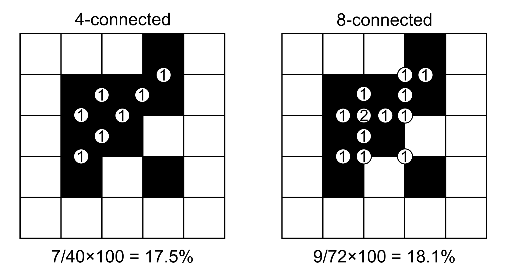
FAC method — FAC computation example on a 5×5 binary input map for both 4- and 8-connectivity. Each circle at a pixel boundary represents an edge pair. A pair scores 1 if both pixels are foreground (FG-FG), and 0 otherwise.#

FED: Foreground Edge Density#

FED computes a weighted measure of foreground involvement in pixel edges. It assigns a partial score to edges where foreground interacts with background, providing a metric that is sensitive to the boundary between foreground and non-foreground areas. The scoring for each pixel pair is:

Foreground–Foreground: 1.0
Foreground–Background: 0.5
Background–Background: 0.0

\[FED = \frac{\text{weighted foreground edges}}{\text{total edges}} \times 100\]

As FAC, the total edges (denominator) depend on window size (W) supporting both 4- and 8-connectivity:

Total edges 4-conn. = \(2 \times W \times (W-1)\)
Total edges 8-conn. = \(2 \times (W-1) \times (2W-1)\)

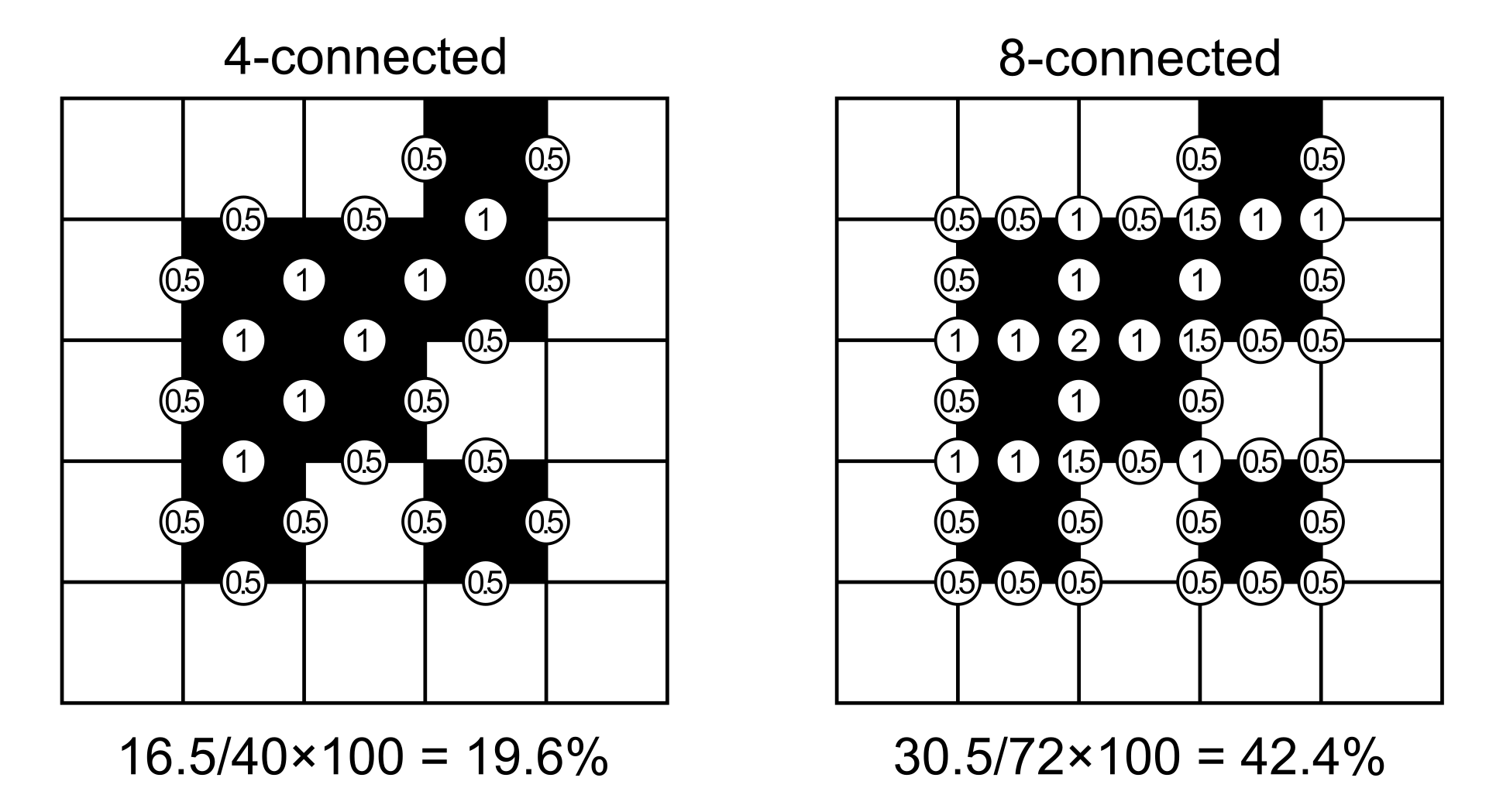
FED method — FED computation example on a 5×5 binary input map for both 4- and 8-connectivity. Each circle shows the weighted score: 1 for FG-FG pairs, 0.5 for FG-BG pairs, and 0 (not shown) for BG-BG pairs. In 8-connected mode, junction points show the sum of both diagonal pairs crossing through them (possible values: 0.5, 1, 1.5, or 2).#

Fragmentation Classes#

The result of a FOS analysis is a map with the same spatial extent as the input, where each foreground pixel receives a value in the range [0, 100] reflecting the FAD or FAC metric in its local neighbourhood. These continuous values are then grouped into 5 classes and colour-coded in the output map:

Foreground cover class	FOS range	Fragmentation	Connectivity
Rare	0 – 10%	Very low	Very high
Patchy	10 – 40%	Low	High
Transitional	40 – 60%	Medium	Medium
Dominant	60 – 90%	High	Low
Interior	90 – 100%	Very high	Very low

Usage#

import pyguidos as pg

# FAD - Foreground Area Density
result = pg.frag(
    in_tiff="my_map.tif",
    method="FAD",
    window_size=27,
    outdir="output/",
    statists=True,
    stat_files=True,
    verb=False
)

# FAC - Foreground Area Clustering (8-connected)
result = pg.frag(
    in_tiff="my_map.tif",
    method="FAC",
    window_size=27,
    connectivity=8
)

# FED - Foreground Edge Density (4-connected)
result = pg.frag(
    in_tiff="my_map.tif",
    method="FED",
    window_size=27,
    connectivity=4
)

Parameters#

Parameter	Type	Default	Description
`in_tiff`	str or Path	–	Path to input GeoTIFF
`method`	str	–	Fragmentation method: `'FAD'`, `'FAC'`, or `'FED'`
`window_size`	int	–	Moving window size in pixels, odd integer >= 3
`connectivity`	int	4	Pixel connectivity for FAC and FED: 4 or 8. Ignored for FAD.
`outdir`	str or Path	None	Output directory
`statists`	bool	True	Compute statistics
`stat_files`	bool	True	Write statistics to files
`verb`	bool	False	Print progress messages

Output Files#

File	Description
`<name>_<method>_<window_size>.tif`	Fragmentation result GeoTIFF with colour palette
`<name>_<method>_<window_size>.txt`	Statistics report
`<name>_<method>_<window_size>.csv`	Per-value pixel counts and frequencies
`<name>_<method>_<window_size>.png`	Foreground pixel histogram

Results#

The frag() function returns a dict. The structure is nested as follows:

output paths (dict or None)
- path tif (str): Absolute path to the fragmentation result GeoTIFF.
- path txt (str): Absolute path to the statistics text report.
- path csv (str): Absolute path to the per-value pixel count CSV.
- path png (str): Absolute path to the foreground pixel histogram image.
- Note: This key is None if stat_files=False.
input stats (dict)
- foreground pxl (int): Count of pixels with value 2 (Forest).
- background pxl (int): Count of pixels with value 1 (Background).
- missing pxl (int): Count of NoData (0) pixels.
- backgr3 pxl (int): Count of special background class 3 pixels.
- backgr4 pxl (int): Count of special background class 4 pixels.
output stats (dict)
- class freq (dict): Breakdown of pixel counts per fragmentation category:
  
  1 rare pxl: Pixels in the “Rare” category.
  
  2 patch pxl: Pixels in the “Patchy” category.
  
  3 trans pxl: Pixels in the “Transitional” category.
  
  4 domin pxl: Pixels in the “Dominant” category.
  
  5 inter pxl: Pixels in the “Interior” category.
- fad_av (float): The average Forest Area Density index.
- avcon (float): The Average Connectivity index.

result = pg.frag("my_map.tif", method="FAD", window_size=27)

# Access statistics
print(result.keys())
# dict_keys(['output paths', 'input stats', 'output stats'])

# Input pixel counts
print(result["input stats"])
# {'foreground pxl': 12500, 'background pxl': 37500, 'missing pxl': 0, ...}

# Fragmentation indices and class pixel counts
print(result["output stats"])
# {{'1 rare pxl': 1200, '2 patch pxl': 2300, '3 trans pxl': 3100,
#  '4 domin pxl': 4200, '5 inter pxl': 1700}, 'fad_av': 62.3, 'avcon': 58.1}

# Output file paths
print(result["output paths"])
# {'path tif': 'output/my_map_frag_fad_27.tif',
#  'path txt': 'output/my_map_frag_fad_27.txt',
#  'path csv': 'output/my_map_frag_fad_27.csv',
#  'path png': 'output/my_map_frag_fad_27.png'}

Computing Statistics Separately#

If you already have a fragmentation output GeoTIFF, you can compute statistics without rerunning the analysis:

stats = pg.frag_stats(
    frag_tiff="output/my_map_frag_fad_27.tif",
    stat_files=True,
    outdir="output/",
    source_tiff="my_map.tif"
)

Note

frag_stats() requires the input GeoTIFF to be an pyGuidos (or GTB) output raster file. See Input Format for details.